Understanding Projections

By Xandamere

If you play DFS, you’ve probably at least seen projections somewhere. You know, those little numbers that seem to say with such confidence that “player A will score X points and.” Maybe there’s even a little value calculation in there that tells you how good or bad of a play that player is based on their salary. How helpful!

Projections are important in DFS, more so in some sports than others. But, despite their widespread availability and use by the DFS community, it’s hard to find information on what a projection actually IS. What does it mean? How is it calculated? Where do those numbers even come from? I’m hoping to help with that here. 

Overview

While every projection system is slightly different, they share common themes so we can “look under the hood” a bit to understand how they’re constructed and that will help us learn how to utilize them effectively. For this exercise, I’m going to primarily use NFL as the example, but the same basic logic applies to projections broadly.

There are a few different areas to explore here, both to understand what a projection is, and to understand how we can utilize them in playing DFS more effectively:

• Projections are median (or occasionally median) outcomes that also assume a normal (or close to normal) distribution of outcomes around the mean.
• Projections also flow from a set of data as well as a set of assumptions, both of which can be flawed.
• In team-based sports, projections do not exist in a vacuum – the actual production of players on the same team is correlated (sometimes positively, sometimes negatively).
• There are limits to projections and we can use our understanding of those limits to make smarter decisions in DFS.

Means, Medians, and Distribution of Outcomes

By default, projection systems are built to show you the mean or median outcome that they project for a given player. Different systems may do it differently here, and most don’t explicitly state whether they’re projecting for mean or median, but generally, most systems are projecting for mean. For the non-math nerds out there, this means the average, roughly. If Tyreek Hill projects for 20 points this week, then if we could travel the multiverse like Dr. Strange and watch this game play out 1,000 times, Tyreek would score around 20,000 total fantasy points in those 1,000 games. 20,000 divided by 1,000 equals 20, thus, a mean projection of 20 fantasy points. So what’s the problem here? Well, as DFS players we don’t generally care all that much about average outcomes. In cash games, we should generally lean towards players who have higher floors, whereas in tournaments, an average outcome isn’t going to help us win anything – we’re going to need ceiling outcomes to take down tournaments. “But wait,” you say, “if one player has a higher mean outcome than another, doesn’t that also mean that player’s ceiling outcomes are higher?” Possibly! But what we also need to care about is that DFS contests don’t take place over a sample of 1,000 games as we used in the previous example. They take place over a sample of 1 game.

Let’s pretend our projections are perfectly accurate for a moment. If Tyreek Hill projects for 20 points and Davante Adams projects for 18 points, in a perfect projection world, we know that over 1,000 games, Tyreek will outscore Davante. But that’s irrelevant to us. The question we need to answer is, over a sample of ONE game, how likely is it that Tyreek outscores Davante? And then we need to consider the ownership of each player, and we need to consider our overall ownership exposure across the entire roster (since we don’t make roster decisions purely in a vacuum), which gets us into the world of game theory and ownership projections – a bit beyond the scope of this piece, but we have lots of content on that subject throughout OWS.

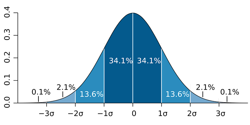
I don’t want to make this crazily math-heavy, so I’ll keep this part simple: if you have a normal distribution with a known standard deviation (Tyreek’s projection), and then you have another distribution with a known standard deviation (Davante’s projection), you can calculate the odds of Davante outscoring Tyreek in a 1-game sample. The problem is, as we’ll dig into in the next section, player outcomes (especially in the NFL with a small sample size of games per season) are not normally distributed! In a normal distribution, roughly 68% of outcomes fall within 1 standard deviation, and 95% of outcomes fall within 2 standard deviations, creating this lovely distribution curve:

Let’s keep picking on Tyreek Hill as our example here. In the 22-23 NFL season, Tyreek averaged 21.6 Draftkings points per game, but with a median points per game of 18. So you can already see one challenge: the mean outcome is quite a bit different from the median outcome. This is because a player can’t really score negative fantasy points; or, at least it’s really, really unlikely – so the distribution skews to the right with mean higher than median for most players (this is critical to prop betting, by the way). If we look at Tyreek Hill’s game logs and then calculate the standard deviation, we get a result of 11 (you can do this yourself if you want – just take a Google Sheet, put in a player’s points per game in a series of cells, and then use the =STDEV(cell range) function to do the math for you).

So what does this mean? It means that, IF fantasy scoring were normally distributed (which it isn’t), we would expect that 68% of the time Tyreek would score between 10.6 and 32.6 Draftkings points. But that is a HUGE range! We’d probably be pretty happy with a 32.6 score in our DFS lineup, but we would definitely not be happy with a 10.6. Now let’s compare Tyreek to Davante. In the 22-23 NFL season, Davante Adams had a mean Draftkings score of 21.1 DK points – about half a point lower than Tyreek. His median was 17.5, also half a point lower than Tyreek. But, the standard deviation of Davante’s scoring was 13.4 – significantly higher than Tyreek, and Davante actually outscored Tyreek in 9 of 17 games. Lower mean, lower median, but he beat Tyreek’s fantasy score (slightly) more than half the time.

Deep threat WRs vs short yard WRs

To perhaps better illustrate this, let’s consider two hypothetical players. One is a deep threat receiver, one is a short-yardage possession receiver. To keep the math simple, let’s say that every time our deep threat receiver gets a catch, it goes for 30 yards and 0.3 touchdowns. Every time our slot receiver gets a catch, it goes for 8 yards and 0.1 touchdowns. In DraftKings scoring, a catch is worth 4.8 points for our deep receiver (1 PPR point + 3 for yardage + 1.8 for touchdown equity, which is 6×0.3). Our possession receiver gets 2.4 points per catch (1 PPR point + 0.8 for yardage and 0.6 for touchdown equity). Now if we project our possession receiver for twice the catches as our deep threat receiver (higher volume for the chain-mover types like Keenan Allen, after all), our two players would have mean point projections that are identical. Following? Cool. But if I ask you who has the higher ceiling, it’s pretty clearly the deep threat receiver, right? The slot receiver’s distribution of outcomes is going to be more tightly clustered around his mean – he’s getting a lot of short, high catch rate targets but without much per-target upside for big plays. The deep threat receiver has the “long bomb for a touchdown” upside, plus with greater per-catch touchdown equity, he has higher odds of a multi-TD game. So, two players can project for exactly the same, but be wildly different plays.

Summary

The picture I’m trying to paint here is that while projections are a useful tool, they are highly imperfect, and understanding their limitations will help make us all better DFS players. The takeaways here:

• Projections are an approximation and do not really tell us as much as we might think about the likelihood of one player outscoring another on any given week.
• Projections are, by default, mean outcomes, but in tournaments, we don’t really care about mean – we care about ceiling (and a player’s chance of hitting it).
• Projections rely on assumptions that are clearly faulty (especially in NFL) because player outcomes are not normally distributed.

Floor and Ceiling

You’ll hear a lot of talk in the DFS space about floor and ceiling, but it’s rare to ever hear anyone actually define what those are. This will be a short section, but I want to at least share how I think about those terms, with the caveat that others may have slightly different definitions when they use these terms.

If you just think about the words, you might think that “floor” means “the lowest score this player can get you,” while “ceiling” would mean “the highest score this player can get you.” But, I would argue that isn’t true, nor would it be helpful even if it is. Every player’s absolute worst outcome is the same: it’s roughly -1 to -2 points (one touch, which they fumble and then never see another touch the rest of the game). The ceiling is a little trickier to define, but we’ve seen enough wild games to think that almost any player COULD feasibly score two or more touchdowns with 100+ yards. So, with these definitions, these terms would just be pretty meaningless to us. So how do we use those terms here at OWS?

As I see it, if you draw a player’s range of outcomes on a chart (which would include that -1 to -2 absolute disaster result!), a player’s floor is somewhere around the 15th-20th percentile. What we’re looking for when we talk about floor isn’t the fewest possible points a player could score, as every player can have the occasional disaster game, but we’re looking for the low range of the most realistic range of outcomes. So if you take a running back who normally sees between 14-24 carries per game (and no targets, because we’re trying to keep this simple), the floor outcome would be 14 carries. Multiply that by 4 yards per carry (roughly the NFL average), assume 0 touchdowns (since we’re talking about the floor – the “bad” outcome), and we get a floor of about 5.6 points (14 carries times 4 yards per carry = 56 yards).

When we’re talking ceiling, we’re looking at the opposite scenario: the 80th-85th percentile outcome. While yes, any given player could possibly benefit from a completely fluky game with multiple broken play 80+ yard touchdowns, we can’t reasonably predict that – that’s not what we’re trying to think about when we build rosters (because any player could have that happen, and there isn’t a great way to predict it). 

Let’s go back to our RB example from before. Now let’s give him 24 carries and assume slightly higher efficiency (say, 5 yards per carry, on the higher end but still within the realm of non-crazy efficiency for NFL running backs), and let’s give him 2 touchdowns (as a yardage and touchdown back, our hero here gets strong goal line equity and 2 TDs is about the most I would ever consider thinking about for a player when considering ceiling). We now get 24X5 yards = 120 yards, 2 TDs, and the 100-yard bonus, which gives us a total of 25 Draftkings points. Our fictional RB now has a normal range of outcomes of between 5.6 – 24 Draftkings points. Now obviously I’m not doing this for every single play on every single slate – that would be ridiculous to calculate by hand – but when making decisions between players that project closely, I try to dig in a little further and look at each player’s range of outcomes for carries & targets, think about touchdown equity, and think about what kind of targets the player sees (short? downfield? Trying to scheme in space where there’s YAC upside?). But Xandamere, you say, some projections HAVE floor and ceiling in them. Can’t I just use that? I mean, OWS has the GPP Ceiling Tool with ceiling projections! True, but I’m always slightly wary of those types of projections because that’s an area where we don’t generally get to see under the hood. A given set of projections might have something for ceiling, but how are they calculating it? With regular projections, I at least have some idea of what’s going into it (which we’ll dive into in the next section), but with floor/ceiling modes, I don’t. I just have to trust whatever the model says, and at least for me, I like understanding how the model works before I place my trust in it. The takeaways:

• “Floor” means 15th-20th percentile outcome, and “ceiling” means 80th-85th percentile outcome.
• You can look at a player’s workload – both volume and type – to build a sense of what a given player’s floor and ceiling looks like. 
• Some projections include floor and ceiling as selectable values. I’m a little wary of those because it’s not really clear how they’re calculated.

How projections are built

Okay, we’ve dug through a lot of background info on some complicated math. Let’s talk about how projections are actually put together. Again, we’ll continue to use NFL as our main example here, but the premise holds for all sports.

Most projection systems are built top-down. What that means is they start with the Vegas total and flow down from there. So, let’s imagine a team is projected to score 24 points – that gives us a sense of touchdown equity (a team with a 24 point total is going to project for something between 2.5 and 3 touchdowns). Then, they will look at play volume, time of possession, and pace for the two teams in the game to figure out the number of plays that each team is likely to run; and then they may look at run/pass play percentages and make some kind of adjustment based on which team is favored (teams that are winning late generally tend to reduce their passing volume, teams that are trailing tend to increase it) to get an adjusted run/pass split. So that looks something like this . . . 

• Two teams are playing. Team A is at home and is favored by 7 points against Team B. Team A has averaged 31 minutes of time of possession and run an average of 66 plays per game, while Team B has also averaged 31 minutes of possession but has run an average of 62 plays per game (they play slower!). So the basic data set here for play volume is 128 plays in 62 minutes of possession, but there aren’t 62 minutes in a game, so when we knock 2 off we end up with something like 124 projected plays in the game. That comes out to something like 64 plays for Team A and 60 for Team B.
• Team A has been passing at a 60% rate but that drops off to 52% when leading, while Team B passes at a 58% rate but that increases to 64% when trailing. Now, these teams won’t be leading or trailing the entire game (and they won’t be leading/trailing by margins large enough to meaningfully impact playcalling tendencies for the entire game), so the full-game numbers might project out to something like a 56% passing play percentage for Team A (as large home favorites) and a 62% passing play percentage for Team B (as road underdogs). That means Team A now projects for 36 dropbacks (64 plays times 0.56) and 28 rush attempts, while Team B now projects for 37 dropbacks and 23 rush attempts.

One word of caution here: don’t just use these splits for prop betting on QB pass attempts, because a dropback doesn’t necessarily end in a pass attempt – sometimes the QB gets sacked, and sometimes they scramble on a non-designed run play. So we can look at sack rates and scramble tendencies, and maybe we now arrive at something like 29 pass attempts for Team A (let’s pretend their QB scrambles a fair bit) and 34 for Team B (their QB is a pocket passer).

Cool, we have play volume! What’s next? Now we look at workload splits for the skill position players to figure out touches/targets. We’ll just hone in on Team B for this one. Remember that Team B has a projection of 23 rush attempts and 34 pass attempts. For the rush attempts, we distribute those between the running backs and whoever else would get a designed run – we have a pocket passer QB, so no designed runs for that poor fellow. Let’s say the team historically gives an RB1 63% of the carries and an RB2 37% (they don’t use an RB3), so now their RB1 projects for 14.5 rush attempts and the RB2 for 8.5 attempts. We do the same for the pass catchers based on their historical volume distribution: maybe 28% for the WR1, 19% for the WR2, 13% for the WR3, 13% for the TE1, 8% for the RB1, 8% for the RB2, and then the other 11% of pass attempts go to a smattering of random rotational dudes. Our WR1 now projects for 8.5 targets, and so on and so forth. Now we know how much volume we can project for each player! We’re making good progress! 

Now we can translate that to fantasy points. We’re just going to stick with the RB1 and the WR1 here, so as not to drown in examples. So we know the RB1 projects for 14.5 rush attempts and 8% of 34 pass attempts, or 2.7 targets. Let’s say that, based on the adjusted line yards matchup and his historical efficiency, RB1 projects for 4.4 yards per carry here. Let’s also say that, because he’s an RB who gets mostly short-yardage dump-offs in the passing game, and he has a 70% catch rate and averages 6 yards per catch. So, our RB1 projects for 63.8 rushing yards (14.5 attempts times 4.4 yards per carry), 1.9 catches, and 11.4 receiving yards. In DK scoring, that’s 6.38 + 1.9 + 1.14 fantasy points, or, 9.42 points. Let’s now say that 40% of the team’s touchdowns have come on the ground and that our RB1 friend has scored 75% of those rushing touchdowns. The team projects for 2 touchdowns (roughly), so that’s 0.8 rushing TDs (2 times 0.4), and our RB1 projects for 0.6 rushing TDs (0.8 total rushing TDs times 0.75 for his 75% share of rushing TDs). A rushing score is worth 6 points, so 0.6 touchdowns is worth 3.6 points. We also know the team projects for 1.2 passing touchdowns (2 total touchdowns minus 0.8 rushing TDs = 1.2 passing TDs), and let’s give the RB1 0.1 of those, for another 0.6 fantasy points. So, our RB1 projects for a total of 9.42 points based on workload/volume, and another 4.2 points based on touchdown equity, for a total projection of 12.62 fantasy points. Cool? Cool.

For the WR1, we know he projects for 8.5 targets. Let’s say he averages a 60% catch rate and 11 yards per catch – that comes out to 5.1 catches for 56.1 yards. Remember that we have 1.2 passing TDs to allocate as well – let’s say the WR1 is also the team’s primary red zone receiving weapon, so even though he only gets 28% of targets, let’s give him 35% of the passing TDs. 35% of 1.2 touchdowns is .42 touchdowns, which is another 2.52 fantasy points. So our WR1 has a projection of 5.1 points for catches, 5.61 points for yardage, and 2.52 points for touchdown equity – he has a projection of 13.23 fantasy points.

Ok, so what’s the point of this? Am I saying you should be doing this math yourself? No, that would be silly – that’s what projections are for! The point here is to learn what goes into projections, under the hood, because that means we have a better understanding of how projections function and how we can use them to make good decisions in DFS.

Team-based projections

The next thing to understand is that projections don’t exist in a vacuum in team-based sports. One player’s production impacts the rest of his team. I’ll use a quick baseball example here because it’s easy and then we’ll go back to NFL: in baseball, let’s pretend you roster a player who hits a home run. Congrats! On Draftkings, a home run is worth at least 14 points. But, what if other guys are on base? Well, now those players come around to score, so anyone on base gets another 2 points for scoring a run. The batter who hit the home run also gets an extra RBI for each man on base, thus an extra 2 points. Baseball is a really clear example of how team scoring flows together (and why stacking is so essential in baseball DFS). If a team does well, it’s generally not just one hitter pounding a bunch of solo HRs, it’s generally multiple guys on the team getting on base, scoring, and driving in runs.

So how does this play out in NFL? Well, remember our projections of Team B (RB1 12.62 fantasy points, WR1 13.23 fantasy points). Let’s say WR1 instead blows past his projections – he gets 8 catches for 125 yards and a touchdown. Happy day for him (and anyone who rostered him in DFS)! What does that do to the rest of the team? Well, there are a couple of possibilities:

• The team could have simply met its overall baseline projections but our WR1 friend just got a larger share of volume (maybe he saw 12 targets instead of his expected 8.5). If our QB has 34 pass attempts and now the WR1 gets 12 targets, that means other guys on the team have to come in under their target projection. In this scenario, WR1’s success negatively impacts the outcome of the rest of his team – the overall pie ends up being the same size, the WR1 just gets a larger share of it than expected.

• The WR1 could also have achieved those results simply based on efficiency. We projected him at 8.5 targets, and so of course he could feasibly land at an 8/125/1 line on that projected volume by achieving a higher than normal catch rate as well as more yards per catch than normal (remember that he averages 11 yards per catch, so 8 catches times 11 yards would be 88 yards).
• But, maybe there was a broken play of some sort, or whatever other random stuff that happens in the NFL, and so he gets an “extra” 37 yards over his projection without negatively impacting volume for the rest of his team. In this scenario, the rest of his team’s skill position projections are unaffected, but we can add roughly an extra point and a half to his quarterback’s projection (37 yards with 1 fantasy point per 25 passing yards), because in this scenario, those 37 extra yards effectively appeared out of thin air – they didn’t come at the expense of volume to other guys.

• The team as a whole could exceed expectations, with multiple guys beating their projections. Remember our sample team here was projected for roughly 2 touchdowns. What happens if they score 3? Or 4? In all likelihood, more touchdowns also mean more offensive yards (because you now have more drives that make it all the way across the field into the end zone), so not only do you have additional touchdown equity across the team’s players, you also have increased yardage. Or, alternately, it means the opposing team turned the ball over multiple times and gave our hero team several short fields, resulting in additional touchdown scoring without necessarily compiling a lot of extra yardage. In this scenario, obviously, the team’s defense/special teams unit gets a boost, as those turnovers generate points for the DST.
  • If we flip the scenario on its head, we can see that other scenarios are also possible. Let’s say our WR1 hero plays like a zero and ends up with a line of 2/22/0. Bummer! Well, either someone else on his team got those yards (if the team met its overall expectations), or, the team as a whole ended up underperforming, dragged down by the poor performance of their top pass catcher.

NBA team projections

Because this is a major part of the piece, I’m also going to talk briefly about NBA here as well. In NBA, you’ll hear people say “there’s only one basketball.” That is, of course, also true for baseball and football, but in both of those sports, scoring can occur in large chunks as a result of single events (a long touchdown, a home run). In basketball, scoring piles up via large numbers of smaller events, and so there only being one basketball is more relevant in basketball than it is in football. Every time one player makes a basket or gets a rebound, that’s a basket or rebound that another player in the game isn’t getting. In MLB and NFL, we think about positive correlation to reduce variance and increase upside in rosters, but in NBA it’s the opposite – we’re more interested in avoiding negative correlation (i.e. it’s incredibly rare for two very expensive players on the same team to both be able to put up tourney-worthy performances in NBA DFS, whereas in MLB DFS it happens all the time and in NFL DFS it can happen with some regularity).

Somewhat complicated, right? That’s okay – the point of this isn’t to suggest that you should be doing calculations around these scenarios, the point is just that you should understand them. Projections don’t exist in a vacuum. If a player outperforms or underperforms their projection, it impacts their team, too – in either a good way or a bad way.

QB and WR pairing rules

In the NFL, broadly speaking, it’s rare that two pass catchers on the same team can put up tourney-viable scores without their quarterback also exceeding expectations. This is the source of the common MME optimizer rule of “at most 1 pass catcher on the same team unless paired with their QB or the opposing QB.” I actually think this is a bad rule, at least in some cases.

While it’s fine in general for putting together game stacks, this rule, in a vacuum, will lead to an optimizer putting together stacks of QB + 1 pass catcher and then having 2 pass catchers from the other team. While this can work (depending on the concentration of volume to the single pass catcher on the QB’s team, if the QB is also a rusher who can run in a score, and the prices of the players involved), there are situations in which it results in dead rosters. For example, let’s say the Lions are playing the Dolphins, and I want to stack that game and I use that rule. I can easily end up with rosters that have, say, Jared Goff + D.J. Chark and then have Tyreek Hill and Jaylen Waddle from the Dolphins. But, at their prices, if both Hill and Waddle put up big games, it’s extremely likely that Tua Tagovailoa materially outscores Goff. This rule is useful in a simplistic sense but be careful with it and think about scenarios where it doesn’t work. Caveat here is that two cheap pass catchers can pay off together without pulling an expensive QB along with them. Price matters! If two pass catchers are both super cheap – say, under $4k on Draftkings, they can both feasibly put up 20 point performances while their QB is hanging around the 18-22 point range.

At OWS, we often say things like “think about the story your roster is telling.” When it comes to stacking and considering using multiple players from the same team, this is what we’re talking about. How outcomes influence projections is one part of that story. Think about it this way: if two players on a team are both projected for good-but-not-huge games, and one of those players fails, it means the other player is more likely to exceed expectations (of course, the entire team could flop – nothing is guaranteed). This is the source of rules like “always 1 Viking” from past years and “1 of Davante Adams and Josh Jacobs from this last season” (highly concentrated offense that usually manage to score points, and so unless outcomes are distributed extremely evenly, someone from the team is highly likely to put up a strong score).

The limits of projections

Projections are a wonderfully useful tool for DFS. They provide numerical representations to thoughts of “who is a good play?” They are useful for identifying players whose likeliest ranges of outcomes are good or bad for their price. But we need to recognize their limits, and we also need to recognize that in 2023, just about every serious DFS player is using them. The point here is that using projections is no longer an edge, it’s just table stakes, and leaning too heavily on them can lead you to overly chalky rosters that have an extremely low chance of taking down a medium to large-sized tournament. We’ll wrap up by summarizing the limits of projections and some takeaways that will, hopefully, be useful going forward:

• Projections are built using mean outcomes, but in tournaments, we care about ceiling. Mean outcomes won’t win you tournaments.
• The best projected players tend to end up with very high ownership, and while how to think about ownership is an entirely separate topic, we can just say here that if you build tournament rosters using mostly high-owned players, your odds of winning a tournament shrink significantly.
• Recognize that while projections are mean outcomes, the range of outcomes around those means will differ from player to player. A short-yardage possession receiver and a deep threat perimeter receiver can both have a projection of 10 DK points but their ranges of outcomes are significantly different.
• Projections are built using a series of historical assumptions around things like passing play rate and market share of carries/targets, but how that plays out in a single game can vary wildly. Teams can take a run heavy or pass heavy approach than can be reasonably projected based on opponent-specific game plans, or what’s expected to happen in that particular game (i.e. if they are leading or trailing by a lot, their playcalling is likely to change a fair bit).
• Projections can’t account for situations such as one pass catcher consistently beating coverage and finding their way into being open and so they receive a much larger than expected share of volume.
• Projections account for “normal” game flows (as predicted by Vegas lines/spreads). If the Vegas implied team totals for a game have the home team at 26 points and the away team at 17 points, the projections are going to be around that (including a higher run rate for the home team and a higher pass rate for the away team). But if the game plays out very differently, projections aren’t really very useful for that. What if the road team jumps out to a big lead early and it changes the game plans for both teams?
• Projections look at historical information to determine the underlying stats for a player (in NFL that’s things like market share of targets, catch rate, yards per catch, etc.), which means they aren’t good at quickly adjusting for a player whose role or ability is changing rapidly. Role changes are easier to account for if someone else on the team is out (i.e. the WR2 steps into the WR1 role), but they aren’t as useful at adjusting to, say, a receiver who has primarily played a perimeter deep threat role shifting over to an X receiver role. They also aren’t very quick to pick up a player whose ability is growing or decreasing, so they’re slow to catch up to young guys breaking out or older players declining.
• Projections don’t tend to do a great job of adjusting for niche matchups. The overall offensive/defensive matchup leads to team totals, which are of course a critical input in projections, but a projection model generally has a tough time adjusting for something like a cornerback matchup or a defense with really large run/pass splits. This is because projections aim for average outcomes. If you’re projecting a team that’s facing an opponent that is 1st in DVOA against the run but 30th against the pass (looking at you, Titans), we might see a smart coach adjust their run/pass play percentage to a large degree to take advantage of that – maybe they go something like 75% pass / 25% run – but projections aren’t going be able to model such an extreme outcome, since they’re aiming for average.
• Overall: projections are useful for looking at normal, expected outcomes across the board, for games, for teams, and for individual players. And in some sports, we see normal outcomes more often (NBA), but in others (NFL, MLB), we see wildly variant outcomes that projections are not effective at accounting for.